Prediction and Motion Forecasting

Prediction estimates how other agents may move over the next few seconds. It is harder than extrapolation because road users respond to maps, signals, social context, hidden intentions, and the ego vehicle's planned motion. A pedestrian near a crosswalk, a cyclist approaching a parked car, and a vehicle edging into an unprotected left turn all require multiple plausible futures rather than one deterministic path.

This page introduces constant-velocity baselines, map-aware trajectory forecasting, social interaction models, multimodal prediction, scene-level prediction, and common datasets. Prediction consumes perception, sensor fusion, and localization/map outputs, then informs behavior planning and motion planning.

Definitions

An agent is a road user whose state and future behavior may affect the ego vehicle: car, truck, bus, motorcycle, pedestrian, cyclist, scooter, emergency vehicle, or construction worker.

A trajectory is a sequence of future states. A simple planar trajectory may be:

$$\tau = \left((x_1,y_1), (x_2,y_2), \ldots, (x_T,y_T)\right).$$

Motion forecasting predicts one or more possible future trajectories for each agent, usually over a horizon of 3 to 8 seconds in driving benchmarks.

Multimodal prediction represents multiple plausible futures. A car at an intersection may go straight, turn left, turn right, or stop. A single averaged trajectory can be physically and behaviorally wrong.

Scene-level prediction models joint futures of multiple agents. This matters because agents interact: one vehicle yields, another proceeds; a pedestrian's crossing decision may depend on ego speed; a merge gap changes as traffic reacts.

Social-LSTM is an early deep model that used recurrent networks and social pooling for pedestrian trajectories. Trajectron++ is a representative graph-structured multimodal forecasting model. Modern AV systems often use graph neural networks, transformers, rasterized BEV encoders, vectorized map encoders, or joint prediction-planning networks.

Argoverse and Waymo Open Motion Dataset are influential motion forecasting datasets. They provide standardized scenarios, agent histories, map context, and future labels for benchmark evaluation.

Key results

A constant-velocity baseline predicts:

$$\hat{p}_{t+k} = p_t + k\Delta t\ v_t.$$

It is simple, transparent, and surprisingly useful over short horizons, especially for vehicles moving steadily in-lane. It fails at stops, turns, merges, yielding, crosswalk behavior, and map-constrained maneuvers.

A constant-acceleration baseline extends the state:

$$\hat{p}_{t+k} = p_t + k\Delta t\ v_t + \frac{1}{2}(k\Delta t)^2 a_t.$$

This can model braking or acceleration but is still weak for intent. A vehicle slowing before an intersection could be stopping, yielding, preparing a turn, or reacting to a pedestrian.

Multimodal predictors often output $K$ trajectories with probabilities:

$$\left\{(\tau^{(1)}, \pi_1), \ldots, (\tau^{(K)}, \pi_K)\right\}, \quad \sum_{k=1}^{K}\pi_k = 1.$$

Evaluation should avoid rewarding averaged futures. Common metrics include average displacement error:

$$\mathrm{ADE} = \frac{1}{T}\sum_{t=1}^{T}\left\|\hat{p}_t-p_t\right\|_2,$$

and final displacement error:

$$\mathrm{FDE} = \left\|\hat{p}_T-p_T\right\|_2.$$

For multimodal outputs, benchmarks often report minADE or minFDE across the best of $K$ modes, sometimes combined with probability calibration. A model that produces many guesses can look good under min error but still be poorly calibrated.

Vectorized scene representations

Forecasting systems need to represent both agent motion and road topology. VectorNet [1] replaced rasterized BEV map images with typed polylines for lanes, crosswalks, stop lines, traffic controls, and agent histories. LaneGCN [2] pushed this further by treating the HD map as a directed lane graph with predecessor, successor, left-neighbor, and right-neighbor edges.

A vectorized scene can be written as:

$$\mathcal{S}=\mathcal{A}_{\mathrm{hist}}\cup\mathcal{M}_{\mathrm{lanes}}\cup\mathcal{M}_{\mathrm{crosswalks}}\cup\mathcal{T}_{\mathrm{signals}}.$$

For a polyline with points $q_0,\ldots,q_m$, consecutive points produce vector tokens:

$$v_i=(q_i,q_{i+1},a_i),$$

where $a_i$ stores type, direction, traffic-light state, timestamp, or polyline id. A local polyline encoder pools vectors belonging to the same entity, then a global graph or attention layer models interactions among lanes and agents:

$$z_p=\mathrm{Attention}(f_p,\{f_q\}_{q=1}^{M}).$$

LaneGCN [2] makes the map topology explicit with relation-specific graph convolution:

$$h_i^{(\ell+1)} =\phi\left(W_0h_i^{(\ell)}+\sum_r\sum_{j\in\mathcal{N}_r(i)}W_rh_j^{(\ell)}\right).$$

Worked example: if lane $L_2$ has successor $L_3$ and left neighbor $L_5$, then straight continuation into $L_3$ and a left lane change into $L_5$ are map-supported modes. A proposed right-lane future is not supported unless the graph also contains a right-neighbor edge. This does not prove the agent will obey the map, but it gives the predictor a strong structural prior.

Hierarchical multi-agent forecasting

Figure: Wayformer compares attention-based encoder-decoder fusion strategies for motion forecasting. From Nayakanti et al., 2022 — embedded under educational fair use with attribution.

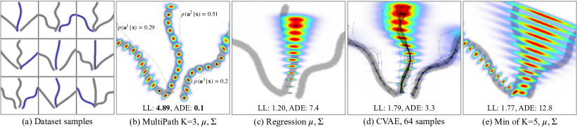
Figure: MultiPath models multimodal future trajectories with fixed anchors, learned offsets, and uncertainty. From Chai et al., 2019 — embedded under educational fair use with attribution.

Target-centric forecasting often normalizes and re-runs the scene once per agent. That is expensive and can produce inconsistent joint futures. HiVT [3] keeps vectorized inputs but separates local context extraction from global interaction: each modeled agent receives a local region of nearby agent and lane vectors, then agent-level context tokens exchange information globally.

The computational motivation is simple. Direct attention over $N$ agents with $T$ history vectors and $L$ lane vectors has token count $NT+L$ and quadratic cost:

$$O((NT+L)^2).$$

A hierarchy compresses local regions first, then performs global attention over roughly $N$ agent tokens. If $N=20$, $T=20$, and $L=300$, direct global attention sees $700^2=490000$ pairwise interactions, while agent-level global attention sees $20^2=400$ pairs. Local work still costs compute, but global scene interaction becomes much cheaper.

HiVT [3] also highlights translation and rotation structure. Displacement features such as $\Delta p_t=p_t-p_{t-1}$ are invariant to global translation, so the model does not need to relearn the same motion at every city coordinate. A planner benefits because it receives multi-agent futures from one shared scene context instead of many isolated per-agent forecasts.

Tracking-aware prediction interfaces

Prediction depends on track continuity. PnPNet [4] put tracking inside an end-to-end trainable perception-prediction subsystem rather than treating it as post-processing after detection. The useful abstraction is a track memory that carries object identity, history, and learned features into the forecasting head.

For a track $q$ and detection $d$, a learned association score can use track features, detection features, spatial displacement, and time gap:

$$s(q,d)=\psi([h_q,h_d,\Delta x,\Delta y,\Delta t]).$$

The tracker updates memory, and the predictor forecasts from trajectory-level actor features:

$$\hat{Y}_i=[(\hat{x}_{i,1},\hat{y}_{i,1}),\ldots,(\hat{x}_{i,T},\hat{y}_{i,T})].$$

Worked example: a vehicle observed at $x=0,2,4$ m at one-second intervals is occluded at $t=3$. A frame-only detector has no current box, but a track memory estimates velocity $2$ m/s, carries the state to $x=6$ m, and forecasts $x=10$ m at $t=5$. That continuity is often the difference between a usable forecast and a flickering object interface.

Prediction is coupled to planning. The ego vehicle's future action changes other agents' futures. If the ego slows, another car may merge; if the ego accelerates, it may not. A purely open-loop predictor can be inconsistent with the planner's chosen trajectory. Interactive prediction and game-theoretic planning address this coupling, but they are harder to validate.

Probability calibration matters. If a predictor assigns 90 percent probability to a crossing pedestrian mode, then over many similar cases that mode should occur about 90 percent of the time. Poorly calibrated probabilities can make planning either timid or reckless. A model with good minFDE but bad calibration may produce one accurate trajectory among many candidates while assigning it the wrong probability.

Prediction horizons should match decisions. A 0.5-second forecast helps emergency braking and cut-in response. A 3-second forecast helps lane changes and intersection yielding. A 7-second forecast may help high-level negotiation but has wide uncertainty. Long-horizon outputs should usually be treated as distributions or intentions, not precise paths. The farther the horizon, the more map topology, traffic rules, and social interaction dominate raw kinematics.

The prediction module should expose uncertainty in a form the planner can use. Covariances, mode probabilities, occupancy over time, reachable sets, and agent intent labels are all possible interfaces. A single polyline without confidence is easy to visualize but often insufficient for safe planning.

Prediction must also represent agents that are only partially observed. A vehicle hidden behind a truck, a pedestrian emerging from between parked cars, or a cyclist occluded by a bus cannot be tracked in the usual way. Some stacks model occlusion zones and generate hypothetical agents from map context and visibility. These hypotheses may have low probability, but they can dominate safety decisions when the ego vehicle is fast or close to the occluded region.

Dataset metrics should be sliced by scenario. A model can have excellent average minADE while performing poorly for unprotected turns, dense crosswalks, emergency vehicles, or unusual road geometry. Useful evaluation reports break down performance by agent class, speed, range, occlusion, map element, weather, and interaction type.

Forecast freshness is another interface requirement: a good old prediction may be less useful than a rough current one when traffic changes quickly.

Visual

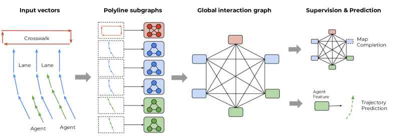
Figure: VectorNet encodes agent histories and HD map elements as polylines before global interaction modeling. From Gao et al., 2020 — embedded under educational fair use with attribution.

This diagram shows two common forecasting architectures at sublayer level. VectorNet builds polyline embeddings and a global graph, while HiVT uses hierarchical temporal, map, local-interaction, and global-interaction attention; both produce multimodal future trajectories with probabilities for planning.

Worked example 1: Constant-velocity forecast

Problem: A tracked car is at position $(x,y)=(12,4)$ m in the ego frame and has velocity $(v_x,v_y)=(8,0)$ m/s. Predict its position after 0.5 s, 1.0 s, and 2.0 s using constant velocity.

1. Use:

$$\hat{p}(t)=p_0+tv.$$

2. At $t=0.5$ s:

$$\hat{p}(0.5)=(12,4)+0.5(8,0)=(16,4).$$

3. At $t=1.0$ s:

$$\hat{p}(1.0)=(12,4)+1.0(8,0)=(20,4).$$

4. At $t=2.0$ s:

$$\hat{p}(2.0)=(12,4)+2.0(8,0)=(28,4).$$

Answer: predicted positions are $(16,4)$ m, $(20,4)$ m, and $(28,4)$ m.

Check: The car advances 8 m each second along $x$ and stays in the same lateral position. If it is approaching a curve or red light, this baseline may become wrong quickly.

Worked example 2: Evaluating two predicted trajectories

Problem: Ground-truth future positions at three seconds are $(5,0)$, $(10,0)$, and $(15,0)$. Predictor A gives $(4,0)$, $(9,0)$, $(14,0)$. Predictor B gives $(5,1)$, $(10,2)$, $(15,3)$. Compute ADE and FDE for both.

1. Predictor A errors at each step:

$$\begin{aligned} e_1 &= \|(4,0)-(5,0)\|=1, \\ e_2 &= \|(9,0)-(10,0)\|=1, \\ e_3 &= \|(14,0)-(15,0)\|=1. \end{aligned}$$

2. Predictor A metrics:

$$\mathrm{ADE}_A = \frac{1+1+1}{3}=1,\quad \mathrm{FDE}_A=1.$$

3. Predictor B errors:

$$\begin{aligned} e_1 &= \|(5,1)-(5,0)\|=1, \\ e_2 &= \|(10,2)-(10,0)\|=2, \\ e_3 &= \|(15,3)-(15,0)\|=3. \end{aligned}$$

4. Predictor B metrics:

$$\mathrm{ADE}_B=\frac{1+2+3}{3}=2,\quad \mathrm{FDE}_B=3.$$

Answer: Predictor A has ADE 1 m and FDE 1 m; Predictor B has ADE 2 m and FDE 3 m.

Check: B becomes increasingly laterally wrong, so its final error is worse. For planning, that may matter if B incorrectly predicts lane occupancy.

Code

import numpy as np

def constant_velocity_forecast(position, velocity, dt, steps):
    times = dt * np.arange(1, steps + 1)
    return position[None, :] + times[:, None] * velocity[None, :]

def ade_fde(pred, truth):
    errors = np.linalg.norm(pred - truth, axis=1)
    return errors.mean(), errors[-1]

pos = np.array([12.0, 4.0])
vel = np.array([8.0, 0.0])
forecast = constant_velocity_forecast(pos, vel, dt=0.5, steps=4)
print(forecast)

truth = np.array([[16.0, 4.0], [20.0, 4.0], [24.0, 4.0], [28.0, 4.0]])
print("ADE, FDE:", ade_fde(forecast, truth))

Common pitfalls

• Averaging incompatible futures. The mean of "turn left" and "go straight" may leave the road.
• Evaluating forecasts without map context. A low ADE path can still violate lane direction, curbs, or traffic rules.
• Assuming independent agents. Merges, unprotected turns, and crosswalks involve coupled decisions.
• Overtrusting long-horizon predictions. Uncertainty grows quickly beyond a few seconds, especially in dense urban scenes.
• Ignoring ego influence. Other agents react to the ego vehicle's speed, position, turn signals, and assertiveness.
• Optimizing benchmark minADE while neglecting probability calibration. Planning needs the likelihood of modes, not only a best-case candidate.

Connections

• Perception, object detection, and segmentation
• Sensor fusion
• Motion planning
• Decision making and behavior planning
• Deep learning
• Reinforcement learning
• Further reading: Social-LSTM, Trajectron++, VectorNet, TNT, LaneGCN, Argoverse forecasting, and Waymo Open Motion Dataset papers.

References

[1] J. Gao, C. Sun, H. Zhao, Y. Shen, D. Anguelov, C. Li, C. Schmid. VectorNet: Encoding HD Maps and Agent Dynamics from Vectorized Representation. CVPR 2020. [2] M. Liang, B. Yang, R. Hu, Y. Chen, R. Liao, S. Feng, R. Urtasun. Learning Lane Graph Representations for Motion Forecasting. ECCV 2020. [3] Z. Zhou, L. Ye, J. Wang, K. Wu, K. Lu. HiVT: Hierarchical Vector Transformer for Multi-Agent Motion Prediction. CVPR 2022. [4] M. Liang, B. Yang, S. Zeng, Y. Chen, R. Hu, S. Casas, R. Urtasun. PnPNet: End-to-End Perception and Prediction with Tracking in the Loop. CVPR 2020.