Perception, Object Detection, and Segmentation

Perception turns raw sensor data into scene understanding: vehicles, pedestrians, cyclists, lanes, drivable space, traffic lights, signs, cones, barriers, and free space. It is the gateway between sensing and action, but it is not a single neural network. Production stacks usually combine 2D image models, 3D lidar or radar models, tracking, map priors, temporal smoothing, uncertainty estimates, and safety monitors.

This page introduces the core perception tasks and metrics that later pages on sensor fusion, prediction, planning, and adversarial attacks build on. The main engineering theme is that perception outputs are not just labels; they are uncertain, delayed, partially observed state estimates used by downstream planners.

Definitions

Object detection localizes and classifies objects. In 2D detection, the output is usually an image bounding box and class label. In 3D detection, the output is a metric box with position, size, heading, class, and confidence in a vehicle, lidar, camera, or global coordinate frame.

Semantic segmentation assigns a class to each pixel or point, such as road, sidewalk, vehicle, vegetation, building, lane marking, or sky. It does not distinguish between separate instances of the same class.

Instance segmentation identifies separate object instances and gives each its own mask. Two adjacent pedestrians receive different instance IDs.

Panoptic segmentation combines semantic and instance segmentation. It labels every pixel or point while distinguishing countable objects, often called "things," from background regions, often called "stuff."

Lane detection estimates lane markings, lane boundaries, lane centerlines, topology, and sometimes lane connectivity through intersections. Lane perception may be image-based, map-assisted, or inferred from trajectories and drivable geometry.

Drivable-area detection estimates where the ego vehicle can physically and legally drive. It can include road surface, lane boundaries, curbs, crosswalks, construction zones, and blocked regions.

IoU, or intersection over union, measures overlap between a predicted region and a ground-truth region:

$$\mathrm{IoU}(A,B) = \frac{|A \cap B|}{|A \cup B|}.$$

Average precision summarizes the precision-recall curve for a class. mAP averages AP across classes and often across IoU thresholds. AV benchmarks may add center-distance thresholds, heading error, velocity error, tracking metrics, or planning-aware scores.

Key results

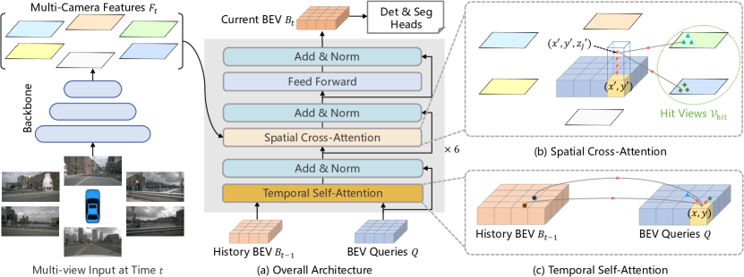
Figure: BEVFormer builds a temporal bird's-eye-view representation from multi-camera image features using transformer attention. From Li et al., 2022 — embedded under educational fair use with attribution.

Figure: DETR3D illustrates how 3D object queries are refined across detection-head layers for camera-only 3D detection. From Wang et al., 2021 — embedded under educational fair use with attribution.

Modern AV perception draws from several detector families. One-stage detectors such as YOLO and RetinaNet directly predict boxes from dense feature maps. Two-stage detectors generate proposals and refine them. Transformer-based detectors such as DETR use set prediction and bipartite matching to avoid hand-designed anchor assignment. 3D lidar detectors such as PointPillars [1] convert point clouds into pseudo-images, while CenterPoint [2] detects object centers in bird's-eye view. Camera-only 3D detection often predicts depth, lifts image features into 3D or BEV, and reasons over multiple cameras and time.

Pillar-based 3D detection

Pillar-based LiDAR detection summarizes each vertical column of a point cloud into one learned feature, then scatters those features into a BEV pseudo-image. PointPillars [1] showed that this representation can avoid expensive 3D convolution while preserving enough road-scene geometry for real-time 3D detection.

If the detection range is divided into ground-plane cells of size $\Delta x \times \Delta y$, a point $(x,y,z,r)$ maps to pillar indices:

$$i=\left\lfloor\frac{x-x_{\min}}{\Delta x}\right\rfloor,\qquad j=\left\lfloor\frac{y-y_{\min}}{\Delta y}\right\rfloor.$$

Each point is decorated with local offsets before pooling, for example:

$$\hat{p}=[x,y,z,r,x-\bar{x}_k,y-\bar{y}_k,z-\bar{z}_k,x-x_k^c,y-y_k^c],$$

where $(\bar{x}_k,\bar{y}_k,\bar{z}_k)$ is the mean point in pillar $k$ and $(x_k^c,y_k^c)$ is the pillar center. The pillar feature is a permutation-invariant pooled point feature:

$$f_k=\max_{n=1,\ldots,N_k}\phi(\hat{p}_{kn}),$$

with the max taken channelwise. After scattering $f_k$ to cell $(i_k,j_k)$, a standard 2D CNN can detect oriented 3D boxes in BEV.

Compact pseudo-code:

for point in lidar_points:
    cell = floor((point.xy - origin_xy) / pillar_size_xy)
    pillars[cell].append(point)

for cell, points in pillars.items():
    decorated = add_mean_and_center_offsets(points, cell)
    feature[cell] = max_pool(shared_mlp(decorated))

bev = scatter(feature)
boxes = detection_head(backbone_2d(bev))

Worked example: with $x \in [0,4)$, $y \in [-2,2)$, and $\Delta x=\Delta y=1$, points $(0.2,-1.4,0.6)$ and $(0.7,-1.1,0.4)$ both fall in pillar $(0,0)$. Their pillar mean is $(0.45,-1.25,0.5)$, so the first point's mean-centered offset is $(-0.25,-0.15,0.10)$. The network sees both absolute position and local shape before it compresses the pillar.

The main tradeoff is vertical compression. Pillars are fast and well matched to road BEV reasoning, but overpasses, stacked objects, steep grades, and unusual vertical structure can be harder to represent when all height variation in one column is summarized by one feature.

Center-based 3D detection and tracking

Figure: CenterPoint reframes 3D detection and tracking around object centers instead of anchor boxes. From Yin et al., 2020 — embedded under educational fair use with attribution.

Anchor-based 3D detectors tile BEV space with many candidate boxes, sizes, and yaw priors. Center-based detectors instead predict object-center heatmaps and regress box attributes only at likely centers. CenterPoint [2] made this idea practical for LiDAR 3D detection and short-term tracking.

For each class $k$, the detector predicts a heatmap:

$$\hat{Y}\in[0,1]^{H\times W\times K},$$

whose local maxima are object centers. At a center cell it regresses:

$$\hat{b}=(\Delta x,\Delta y,z,w,l,h,\sin\theta,\cos\theta,v_x,v_y).$$

The offsets correct feature-stride quantization, $(w,l,h)$ and $z$ reconstruct the 3D box, $\sin\theta,\cos\theta$ avoid the yaw discontinuity at $\pm\pi$, and velocity supports tracking. A Gaussian target around the annotated center gives smoother supervision than a single positive pixel:

$$Y_{xyk}=\exp\left(-\frac{(x-q_x)^2+(y-q_y)^2}{2\sigma^2}\right).$$

Worked example: suppose the output stride is $0.5$ m, the grid origin is $(0,-20)$ m, and a car center is $(12.3,-4.1)$ m. The grid coordinates are $(24.6,31.8)$, so the heatmap peak is at cell $(24,31)$ and the offset target is $(0.6,0.8)$. Multiplying the offset by stride restores the metric correction $(0.3,0.4)$ m.

For short-term tracking, a detected center $c_t$ with predicted velocity $\hat{v}$ can be projected to the previous frame:

$$\hat{c}_{t-1}=c_t-\hat{v}\Delta t.$$

The tracker links this projected center to a nearby previous track. This is not a full tracking theory, but it is a useful perception interface: detection, velocity, and track association all operate on the same center representation.

The precision-recall tradeoff matters more than raw accuracy. Precision is:

$$\mathrm{precision} = \frac{\mathrm{TP}}{\mathrm{TP}+\mathrm{FP}},$$

and recall is:

$$\mathrm{recall} = \frac{\mathrm{TP}}{\mathrm{TP}+\mathrm{FN}}.$$

For planning, false negatives can hide real hazards, while false positives can cause unnecessary braking or stuck behavior. The best operating point depends on object type, range, speed, and maneuver. Missing a pedestrian in the lane is much worse than temporarily over-segmenting a bush near the sidewalk, but persistent false obstacles can still create unsafe traffic interactions.

3D boxes need coordinate discipline. A predicted box may be represented by center $(x,y,z)$, dimensions $(l,w,h)$, yaw $\theta$, velocity $(v_x,v_y)$, class $c$, and confidence $p$. The downstream planner needs to know the frame, timestamp, and covariance or confidence calibration. A 3D box with the right label but the wrong timestamp can be operationally wrong.

Temporal perception reduces flicker. A single frame may miss an occluded cyclist or misread a traffic light under glare. Tracking, recurrent networks, temporal transformers, and multi-frame BEV encoders allow the system to maintain hypotheses over time. Temporal smoothing, however, can also preserve stale objects after the scene changes, so deletion logic and uncertainty growth are important.

Lane and drivable-area perception are not solved by local image edges alone. Intersections, faded markings, snow, construction, reversible lanes, temporary traffic control, and emergency worker gestures often require map context, semantics, traffic rules, and behavioral reasoning.

Open-set perception is a practical requirement. The road contains objects outside a fixed label taxonomy: fallen cargo, unusual trailers, temporary barriers, animals, hand signals, flooded lanes, and damaged infrastructure. A detector may not know the exact class, but the stack still needs to represent occupancy, motion, size, and risk. Unknown-object handling is one reason occupancy and free-space estimation remain important alongside named-object detection.

Perception outputs also need lifecycle management. A detection becomes a track, a track accumulates history, and stale tracks must be deleted when evidence disappears. Deleting too aggressively causes flicker; deleting too slowly leaves phantom obstacles. This tradeoff is central to usable AV perception.

Visual

Figure: PointPillars converts sparse point clouds into pillar features before 2D convolutional detection. From Lang et al., 2019 — embedded under educational fair use with attribution.

This diagram expands perception into the standard camera, PointPillars/CenterPoint, VoxelNet, and radar branches. The key shape transition is from unordered lidar points to voxels/pillars and then to a BEV tensor, while the downstream association block turns raw detections into tracked objects and uncertainty for prediction and planning.

Worked example 1: Computing IoU for two boxes

Problem: A ground-truth 2D box spans $x = 10$ to $50$ and $y = 20$ to $60$. A detector predicts $x = 30$ to $70$ and $y = 40$ to $80$. Compute IoU.

1. Compute ground-truth area:

$$A_{\mathrm{gt}} = (50-10)(60-20)=40 \times 40=1600.$$

2. Compute predicted area:

$$A_{\mathrm{pred}} = (70-30)(80-40)=40 \times 40=1600.$$

3. Compute intersection limits:

$$\begin{aligned} x_{\min} &= \max(10,30)=30, \\ x_{\max} &= \min(50,70)=50, \\ y_{\min} &= \max(20,40)=40, \\ y_{\max} &= \min(60,80)=60. \end{aligned}$$

4. Intersection width and height are $20$ and $20$, so:

$$A_{\cap}=20 \times 20=400.$$

5. Union area is:

$$A_{\cup}=1600+1600-400=2800.$$

6. IoU is:

$$\mathrm{IoU}=\frac{400}{2800}=0.1429.$$

Answer: IoU is about 0.143. At a 0.5 IoU threshold this prediction is not a true positive, even though the boxes overlap visually.

Worked example 2: Precision and recall for pedestrian detection

Problem: In a validation slice, there are 20 labeled pedestrians. A detector reports 25 pedestrian boxes. Of those, 15 match true pedestrians at the required IoU threshold. Compute precision and recall.

1. True positives are matched detections:

$$\mathrm{TP}=15.$$

2. False positives are reported boxes that do not match:

$$\mathrm{FP}=25-15=10.$$

3. False negatives are labeled pedestrians missed by the detector:

$$\mathrm{FN}=20-15=5.$$

4. Compute precision:

$$\mathrm{precision}=\frac{15}{15+10}=0.60.$$

5. Compute recall:

$$\mathrm{recall}=\frac{15}{15+5}=0.75.$$

Answer: precision is 60 percent and recall is 75 percent.

Check: The detector found three quarters of real pedestrians but produced many extra detections. A downstream planner might tolerate extra detections at low speed but not repeated phantom braking at highway speed.

Code

import numpy as np

def box_iou_xyxy(a, b):
    xa1, ya1, xa2, ya2 = a
    xb1, yb1, xb2, yb2 = b
    ix1, iy1 = max(xa1, xb1), max(ya1, yb1)
    ix2, iy2 = min(xa2, xb2), min(ya2, yb2)
    iw, ih = max(0.0, ix2 - ix1), max(0.0, iy2 - iy1)
    inter = iw * ih
    area_a = max(0.0, xa2 - xa1) * max(0.0, ya2 - ya1)
    area_b = max(0.0, xb2 - xb1) * max(0.0, yb2 - yb1)
    union = area_a + area_b - inter
    return 0.0 if union == 0.0 else inter / union

def greedy_match(pred_boxes, gt_boxes, threshold=0.5):
    used_gt = set()
    matches = []
    for i, pred in enumerate(pred_boxes):
        scores = [(box_iou_xyxy(pred, gt), j) for j, gt in enumerate(gt_boxes) if j not in used_gt]
        if not scores:
            continue
        score, j = max(scores)
        if score >= threshold:
            used_gt.add(j)
            matches.append((i, j, score))
    return matches

pred = np.array([[30, 40, 70, 80], [100, 100, 130, 160]])
gt = np.array([[10, 20, 50, 60], [98, 96, 132, 161]])
print(greedy_match(pred, gt, threshold=0.5))

Common pitfalls

• Reporting mAP without showing operating points. A planner needs thresholded behavior, not only benchmark summaries.
• Ignoring calibration of confidence scores. A detector that says 0.9 confidence should be right roughly 90 percent of the time in comparable conditions if downstream modules treat confidence probabilistically.
• Evaluating only clear-weather daytime data. Night, rain, glare, construction, unusual vehicles, and occlusion dominate safety risk.
• Treating segmentation as truth. Pixel masks can be crisp but semantically wrong, especially on reflective surfaces, shadows, snow, and road debris.
• Forgetting temporal latency. A high-quality detection that arrives too late can be worse than a noisier but timely estimate.
• Overfitting to benchmark taxonomies. Real roads contain objects outside the training label set, such as fallen cargo, temporary signs, animals, and hand gestures.

Connections

• Sensors, cameras, lidar, radar, and IMU
• Depth estimation and stereo vision
• Sensor fusion
• Prediction and motion forecasting
• Deep learning
• Adversarial attacks on AV perception
• Further reading: YOLO, RetinaNet, DETR, PointPillars, CenterPoint, Mask R-CNN, Panoptic FPN, and nuScenes or Waymo Open Dataset benchmark papers.

References

[1] A. H. Lang, S. Vora, H. Caesar, L. Zhou, J. Yang, O. Beijbom. PointPillars: Fast Encoders for Object Detection from Point Clouds. CVPR 2019. [2] T. Yin, X. Zhou, P. Krahenbuhl. Center-based 3D Object Detection and Tracking. CVPR 2021.